Chapter 5 Repeated Measures Design
5.1 Repeated measures design
- Motivation for repeated measures
- Sampling scheme
- Estimation, hypothesis, and causal interpretation
- Split plot design
- Longitudinal data
- Experiments
- Observational studies: prospective and retrospective cohort study
- Sampling scheme for observational studies
5.2 Analysis of repeated measures designs
5.2.1 Two-way ANOVA model
- Model
- Estimators
- Sum of squares and mean squares
- Statistical inference
- Hypothesis testing
- Confidence intervals
5.2.2 More complicated repeated measures design
- Two factors with repeated measures on one factor
- Two factors with repeated measures on both
- Split-plot design
For more discussion, see Chapter 8 here.
5.2.3 Longitudinal data analysis
We consider the rat growth data. Each rat is measured over 5 weeks. This type of data set is called longitudinal since the observations are taken over time. There is a covariate “mother’s weight” (X). The idea is to see how rat weights vary over time since birth. In another example, logarithm of CD4 counts are listed for patients on three different treatments over time. Goal is to investigate how CD4 counts change over time and if age has any effect on this change. Note that in the first example, the times at which measurement are taken are the same for all subjects. In the second case times may be different for different patients.
Rat.growth <- read.csv(file="./data/Growth.csv", header=TRUE, sep=",")

colorpicks = rainbow(n=length(unique(Rat.growth$rat)));
with(Rat.growth, plot(y=weight, x=week,type='p', pch=16, bty='l',  main='Raw growth data', xlab='Week', ylab='Weight',col=colorpicks[rat]))
for(i in 1:length(unique(Rat.growth$rat))){
  one.rat=Rat.growth[Rat.growth$rat==i,]
  with(one.rat, lines(weight, week,col=colorpicks[rat]))
}
# For more thoughts on visualization, see http://www.colbyimaging.com/wiki/statistics/longitudinal-data
legend('bottomright', col=colorpicks, pch=c(16), legend=paste('Rat', unique(Rat.growth$rat)))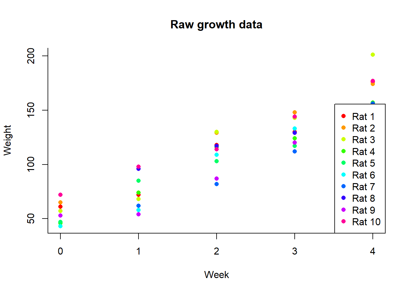
We consider several models to fit them in R. For more on the syntax of lmer see the vignette here.
library(lme4)
lm1=lmer(weight~as.factor(week)+(1|rat),data=Rat.growth)
lm2=lmer(weight~week+X+(1|rat),data=Rat.growth)
lm3=lmer(weight~as.factor(week)+X+(1|rat),data=Rat.growth)
lm4=lmer(weight~week+X+(1|rat)+(0+week|rat),data=Rat.growth)
lm5=lmer(weight~week+I(week^2)+X+(1|rat),data=Rat.growth)
lm6=lmer(weight~week+I(week^2)+X+(1|rat)+(0+week|rat)+(0+week^2|rat),data=Rat.growth)
# For model selection, we can use AIC, BIC
AIC(logLik(lm1))## [1] 380# or
AIC(lm1,lm2)## df AIC
## lm1 7 380
## lm2 5 390BIC(lm1,lm2,lm3,lm4,lm5,lm6)## df BIC
## lm1 7 393
## lm2 5 400
## lm3 8 389
## lm4 6 404
## lm5 6 401
## lm6 8 4095.3 Learning Objectives
- Students can recognize repeated measures designs.
- Students understand the basics of cohort studies.
- Students can fit random effects model in
R.